Data reduction using variance threshold, univariate feature selection, recursive feature elimination, PCA
This blog is about how we perform data reduction using variance threshold, univariate feature selection, recursive feature elimination, PCA.
For this tutorial, I am using the Iris dataset.
First of load all necessary libraries for this tutorial.

Now, load the Iris dataset.

Let’s find the shape of the Iris dataset.

The data has four features. To test the effectiveness of different feature selection methods, we add some noise features to the data set.

Before applying the feature selection method, we need to split the data first. The reason is that we only select features based on the information from the training set, not on the whole data set.

Variance Threshold
Variance Threshold is a feature selector that removes all low-variance features. This feature selection algorithm looks only at the features (X), not the desired outputs (y), and can thus be used for unsupervised learning. Features with a training-set variance lower than this threshold will be removed.

Univariate Feature Selection
Univariate feature selection works by selecting the best features based on univariate statistical tests. We compare each feature to the target variable, to see whether there is any statistically significant relationship between them. It is also called the analysis of variance (ANOVA). That is why it’s called ‘univariate’.
f_classif

2. chi2

3. mutual_info_classif

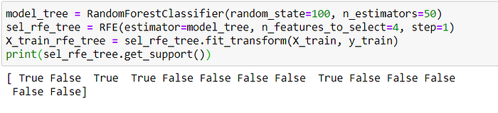
Recursive Feature Elimination
Recursive feature elimination (RFE) is a feature selection method that fits a model and removes the weakest feature (or features) until the specified number of features is reached. RFE requires a specified number of features to keep. However, it is often not known in advance how many features are valid.
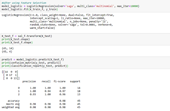
Differences Between Before and After Using Feature Selection
a. Before using feature selection:

b. After using feature selection:
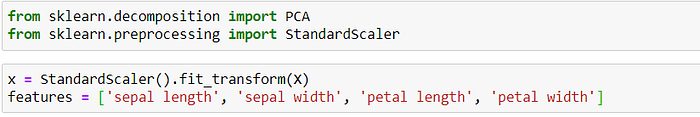
Principal Component Analysis (PCA)
The principal components of a collection of points in real coordinate space are a sequence of p unit vectors, where the i-th vector is the direction of a line that best fits the data while being orthogonal to the first i-1 vectors.
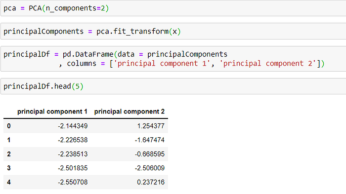
PCA Projection to 2D
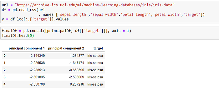
The original data has four columns (sepal length, sepal width, petal length, and petal width). In this section, the code projects the original data which is 4-dimensional into 2 dimensions. The new components are just the two main dimensions of variation.
Concatenating DataFrame along axis = 1. finalDf is the final DataFrame before plotting the data.
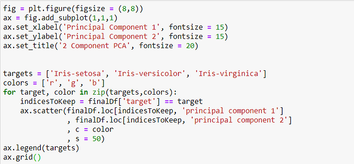
Now, let’s visualize the DataFrame. Execute the following code:

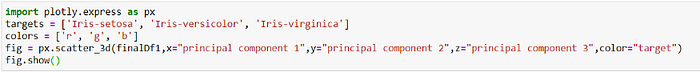
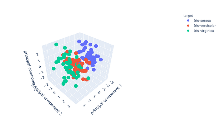
Now let’s visualize the 3D graph:
Thank You!
